A month ago, I finished a seminar paper for the Mathematical Statistics course in my master’s program at the University of Belgrade, School of Electrical Engineering, titled \(f\)-divergences: hypothesis testing, inequalities and statistical estimation. This post is where I write down what I learned while researching and writing it, so that I don’t forget it, and so that others can get something out of it too. The paper itself is in Serbian, which is one more reason I couldn’t just share it as is. So this isn’t a translation but a retelling: shorter, less formal, and focused on what these ideas mean for machine learning. A few parts, especially the practical ones in Sections 6 and 7, weren’t in the paper at all.
I picked the topic for a selfish reason. I work with flow matching [1], and the generative modeling literature is full of divergences. Maximum likelihood “minimizes KL” [2]. The OG GAN “minimizes Jensen–Shannon” [3]. Wasserstein GANs exist because the other divergences “saturate” [4], [5]. RLHF adds a “KL penalty” [6], [7]. Flow matching talks about “optimal transport paths” [1], [8]. I could follow these sentences, but I didn’t really understand why these particular quantities show up, what they have in common, and where each of them breaks. Writing the paper was my way of strengthening that part of my mathematical foundation.
If you remember one thing from this post, make it this: an \(f\)-divergence looks at the likelihood ratio \(p(x)/q(x)\) at every point and averages a convex penalty of it. Almost everything below follows from that one sentence: the nice properties, the connection to classifiers, Fisher information, the KL estimators used in RLHF, and the failure that motivates Wasserstein distances.
I won’t prove everything. Where a proof is short or teaches something, I sketch it; otherwise I state the result and point to the references. The main reference throughout is the book by Polyanskiy and Wu [9].
1. A test statistic that was secretly a divergence
Comparing two probability distributions is one of the basic problems in statistics. We need some number that says how much a distribution \(P\) differs from a distribution \(Q\). Formally, a divergence is any map that assigns such a number \(D(P\|Q) \ge 0\) to every pair of distributions, with \(D(P\|Q) = 0\) if and only if \(P = Q\) [9]. Unlike a distance, a divergence doesn’t have to be symmetric or satisfy the triangle inequality.
Historically, the classic divergences weren’t derived from one general definition. Each was invented separately, for its own problem: Pearson’s statistic for testing discrete distributions, the Kolmogorov–Smirnov and Cramér–von Mises statistics for continuous ones, and the Kullback–Leibler divergence in information theory. Only in the 1960s did Csiszár [10] and, independently, Ali and Silvey [11] notice that most of them are special cases of one construction.
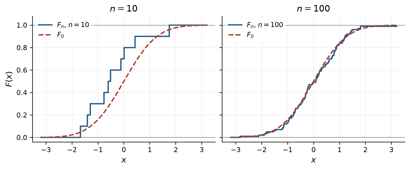
The nicest way I found into the topic is the classic goodness-of-fit problem. Given a sample \(X_1, \dots, X_n\), we want to test whether it comes from a hypothesized distribution \(F_0\). The natural estimate of the unknown CDF is the empirical CDF
and the Glivenko–Cantelli theorem says that \(F_n\) converges to the true CDF uniformly, almost surely: \(\sup_x |F_n(x) - F(x)| \to 0\) [12]. You can see this in Figure 1. So \(F_n\) is a legitimate estimate of the distribution, and the gap between \(F_n\) and \(F_0\) can be read as an estimate of a distance between distributions, not just random noise. The question is how to measure that gap.
The oldest answer is Pearson’s \(\chi^2\) test. Split the real line into \(r\) bins \(A_1, \dots, A_r\), let \(p_{j0}\) be the probability of bin \(j\) under \(F_0\), and let \(N_j\) be the number of sample points that fall into it. Pearson’s statistic is [12]
Now define the \(\chi^2\)-divergence between two discrete distributions \(p\) and \(q\) as \(\chi^2(p\|q) = \sum_j (p_j - q_j)^2 / q_j\). Substituting the empirical frequencies \(\hat p_j = N_j / n\) gives
So, a statistic we had only ever used as a recipe is exactly \(n\) times a divergence between the empirical distribution and the hypothesized one.
This is also how the test works. If the sample really does come from \(F_0\) (the null hypothesis), then for large \(n\) the statistic behaves like a random variable with the \(\chi^2\) distribution with \(r - 1\) degrees of freedom. It’s one less than the number of bins because the counts must add up to \(n\), so only \(r - 1\) of them can vary freely. You compute the statistic, compare it with, say, the 95th percentile of the \(\chi^2(r-1)\) distribution, and reject \(F_0\) if it’s larger: a divergence that big would be unlikely if \(F_0\) were true.
The Kolmogorov–Smirnov statistic \(\sqrt{n}\,\sup_x |F_n(x) - F_0(x)|\) and the Cramér–von Mises statistic \(n \int (F_n - F_0)^2\, dF_0\) compare CDFs, not densities or probabilities at individual points. As we’ll see, that means they are not \(f\)-divergences. Keep them in mind; they come back in Section 7.3.
2. \(f\)-divergences
2.1 The definition
Let \(f : (0, \infty) \to \mathbb{R}\) be a convex function with \(f(1) = 0\). The \(f\)-divergence of \(P\) from \(Q\) is [9]
with a sum instead of the integral for discrete distributions. In full generality, \(p/q\) is replaced by the Radon–Nikodym derivative \(dP/dQ\), which also covers distributions without densities, but the intuition is the same.
The quantity \(r(x) = p(x)/q(x)\) is the likelihood ratio: how many times more likely the point \(x\) is under \(P\) than under \(Q\). If the distributions agree, \(r \equiv 1\). The condition \(f(1) = 0\) says “no penalty where the distributions agree”, and convexity says that large deviations of \(r\) from \(1\) cost disproportionately more. The divergence is the average penalty, weighted by \(Q\).
Why is this always nonnegative? It’s a one-line application of Jensen’s inequality, and it’s the whole reason the definition works. Since \(\mathbb{E}_Q[r(X)] = \int p = 1\),
If \(f\) is strictly convex at \(1\), equality forces \(r\) to be constant, hence \(r \equiv 1\) and \(P = Q\) [9].
Two details that will matter later:
- \(f\) is not unique. Adding \(c(t-1)\) to \(f\) doesn’t change the divergence, because \(\mathbb{E}_Q[r - 1] = 0\). This looks like a technicality, but in Section 6.5.3 it turns out to be exactly the trick behind the best KL estimator used in RLHF.
-
What if \(q(x) = 0\) but \(p(x) > 0\)? Then the ratio \(p/q\) is infinite, and the term \(q\, f(p/q)\) has the form \(0 \cdot \infty\). The natural value is its limit as \(q\) shrinks to zero. Writing \(t = p/q\), so that \(q = p/t\),
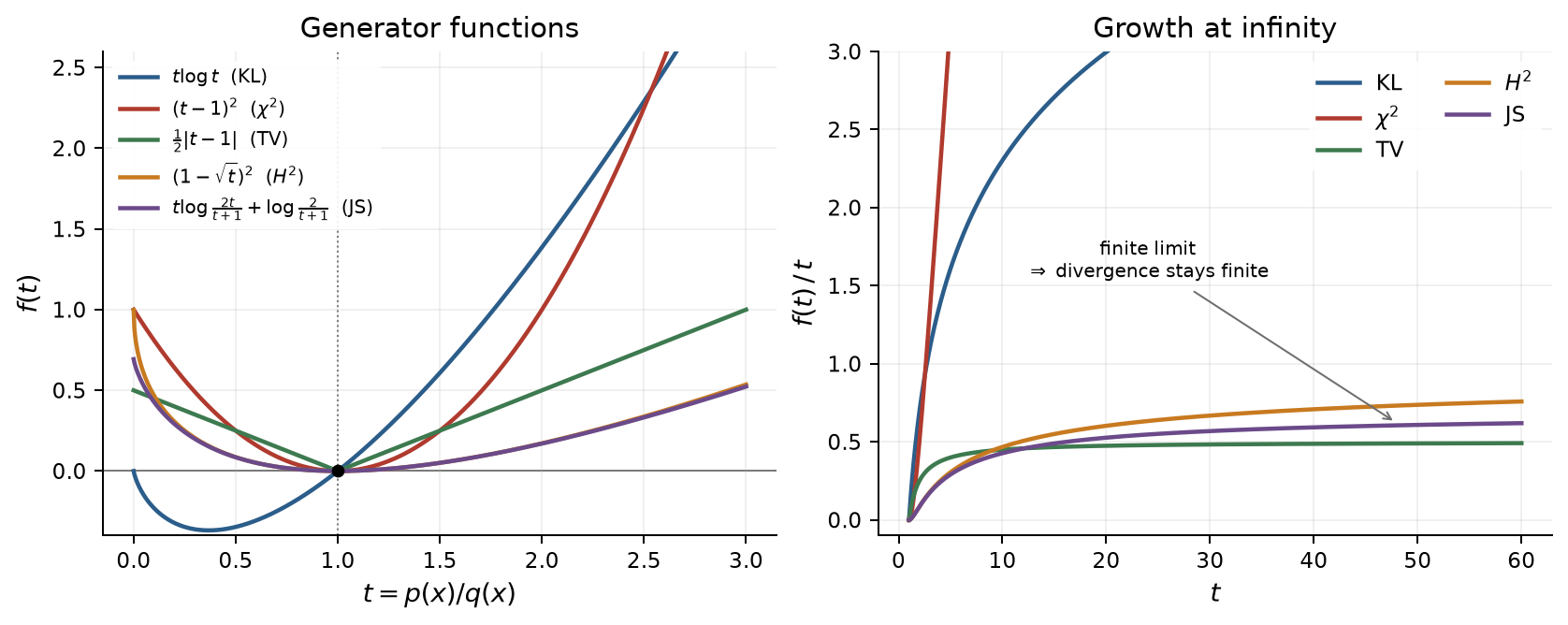
\[ q\, f\!\left(\frac{p}{q}\right) = p\, \frac{f(t)}{t} \;\longrightarrow\; p \cdot \lim_{t \to \infty} \frac{f(t)}{t} \qquad (q \to 0,\ t \to \infty). \]So everything depends on how fast \(f\) grows. For KL, \(f(t)/t = \log t \to \infty\), and for \(\chi^2\), \(f(t)/t \approx t \to \infty\): if \(P\) puts any mass where \(Q\) has none, the divergence is infinite. For total variation, Hellinger and Jensen–Shannon, \(f\) grows at most linearly, so \(f(t)/t\) levels off at a finite value (\(\tfrac12\), \(1\) and \(\log 2\)) and the divergence stays finite. The right panel of Figure 2 shows exactly this.
2.2 The usual suspects
Different choices of \(f\) give the classic divergences:
| Divergence | \(f(t)\) | Symmetric | Range |
|---|---|---|---|
| Kullback–Leibler \(\mathrm{KL}(P\|Q)\) | \(t \log t\) | no | \([0, +\infty]\) |
| \(\chi^2\)-divergence \(\chi^2(P\|Q)\) | \((t-1)^2\) | no | \([0, +\infty]\) |
| Total variation \(\mathrm{TV}(P,Q)\) | \(\tfrac12 \lvert t-1 \rvert\) | yes | \([0, 1]\) |
| Squared Hellinger \(H^2(P,Q)\) | \((1-\sqrt t)^2\) | yes | \([0, 2]\) |
| Jensen–Shannon \(\mathrm{JS}(P,Q)\) | \(t\log\frac{2t}{t+1} + \log\frac{2}{t+1}\) | yes | \([0, 2\log 2]\) |
Figure 2 plots these generators. They’re all convex and all pass through \((1, 0)\); what tells them apart is how fast they grow, which decides whether the divergence can be infinite.
Here’s what each one measures. In every case, the formula comes from plugging that row’s \(f\) into the definition \(D_f(P\|Q) = \int q\, f(p/q)\).
2.2.1 KL divergence
With \(f(t) = t \log t\), the \(q\) cancels:
It’s the average log-likelihood ratio when the data really comes from \(P\): how surprised, on average, you’d be by samples from \(P\) if you believed they came from \(Q\). In information theory, it’s the expected number of extra bits (or nats, with the natural log) you waste by encoding samples from \(P\) with a code designed for \(Q\). Note that the average is taken under \(P\), so KL mostly cares about the places where \(P\) has mass. This makes it strongly asymmetric: if \(Q\) gives zero probability to something \(P\) can produce, \(\mathrm{KL}(P\|Q) = \infty\), while \(\mathrm{KL}(Q\|P)\) can still be finite. Section 2.3 shows why this matters so much in ML.
2.2.2 χ²-divergence
With \(f(t) = (t-1)^2\),
where the last step uses \(\mathbb{E}_Q[p/q] = 1\). So \(\chi^2\) is simply the variance of the likelihood ratio. This is Pearson’s divergence from Section 1, and in ML it shows up whenever you reweight samples: if you estimate an expectation under \(P\) using \(n\) samples from \(Q\) and importance weights \(p/q\) (as in off-policy RL), your effective sample size is roughly \(n / (1 + \chi^2(P\|Q))\). Because of the division by \(q\), it’s extremely sensitive to places where \(Q\) has little mass. In Section 5 it will turn out to describe the local behavior of every smooth \(f\)-divergence.
2.2.3 Total variation
With \(f(t) = \tfrac12 |t - 1|\),
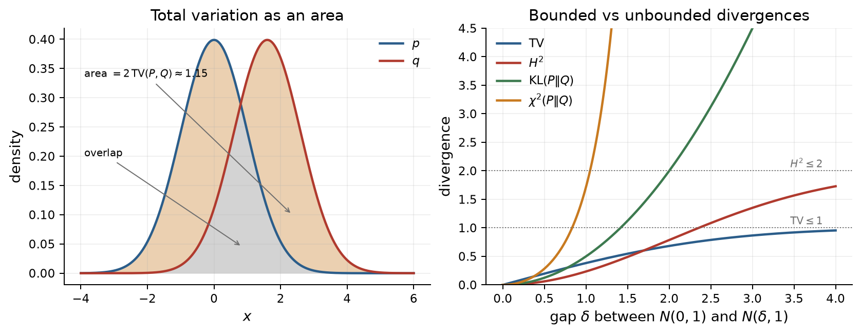
which is half the area between the two densities (left panel of Figure 3). Equivalently, it’s the largest amount by which the two distributions can disagree about the probability of any single event, \(\sup_A |P(A) - Q(A)|\), attained by the event \(A = \{x : p(x) > q(x)\}\). It’s always between \(0\) and \(1\), it equals \(1\) exactly when the two distributions don’t overlap at all, and it’s symmetric and satisfies the triangle inequality, so it’s a true distance. Some texts drop the \(\tfrac12\) and use \(f(t) = |t - 1|\), which gives \(\int |p - q|\) with values in \([0, 2]\); this post keeps the \(\tfrac12\) throughout, following [9]. Section 3 shows it measures exactly how well the best possible classifier can tell \(P\) and \(Q\) apart.
2.2.4 Squared Hellinger distance
With \(f(t) = (1 - \sqrt t)^2\),
So it’s the squared Euclidean distance between the square roots of the densities. The integral \(\int \sqrt{pq}\), called the Bhattacharyya coefficient, measures overlap: it’s \(1\) when the distributions are identical and \(0\) when they don’t overlap, so \(H^2\) lies between \(0\) and \(2\) (right panel of Figure 3). Its practical superpower is independence: for \(n\) i.i.d. samples, the overlap simply multiplies, \(\int \sqrt{p^n q^n} = \left(\int \sqrt{pq}\right)^n\). That gives an exact formula for the Hellinger distance between the distributions of \(n\) samples, which is why it’s a standard tool in asymptotic statistics. (Total variation, by contrast, has no such formula.)
2.2.5 Jensen–Shannon divergence
The generator in the table looks scary, but it’s equivalent to a much friendlier form: compare both distributions to their average \(M = \tfrac12 (P + Q)\),
It’s symmetric by construction, and it’s always finite. Since \(m = \tfrac12 (p + q) \ge \tfrac12 p\), the ratio \(p/m\) is never larger than \(2\), so each KL term is at most \(\log 2\). It’s also the divergence behind the original GAN: with the optimal discriminator, the generator minimizes \(-\log 4 + \mathrm{JS}(P_{\text{data}}, P_G)\) [3]. (Many ML papers put a factor of \(\tfrac12\) in front, which changes the range to \([0, \log 2]\). I’m following the convention from my seminar paper.)
2.3 Forward vs reverse KL
The asymmetry of KL matters a lot in machine learning, so it’s worth a short detour. Take a model \(P_\theta\) with density \(p_\theta\), and data from a distribution \(P_{\text{data}}\) with density \(p_{\text{data}}\). Maximum likelihood training maximizes the average log-likelihood of the dataset, \(\frac1N \sum_{i=1}^N \log p_\theta(x_i)\), which by the law of large numbers estimates \(\mathbb{E}_{x \sim P_{\text{data}}}[\log p_\theta(x)]\). The trick for seeing what this expectation measures is to add and subtract \(\log p_{\text{data}}(x)\) inside it:
The first term is minus the entropy of the data, \(H(P) = -\mathbb{E}_{X\sim P}[\log p(X)]\), and the second is exactly the KL formula from Section 2.2.1. The entropy depends only on the data, not on \(\theta\). So maximum likelihood is exactly minimizing the forward KL \(\mathrm{KL}(P_{\text{data}}\|P_\theta)\). The same identity, read with a minus sign, says that the cross-entropy loss we minimize when training classifiers and language models is \(H(P_{\text{data}}) + \mathrm{KL}(P_{\text{data}}\|P_\theta)\): an irreducible part set by the data, plus a KL part that training can shrink. Since KL is never negative, no model can get its loss below the entropy of the data.
Now look at which mistakes the forward KL punishes. Its integrand \(p_{\text{data}} \log(p_{\text{data}}/p_\theta)\) explodes wherever the data has mass and the model doesn’t, so the model is forced to cover every mode of the data, even if that means putting mass in between them. This is called mode-covering. The reverse KL, \(\mathrm{KL}(P_\theta\|P_{\text{data}}) = \mathbb{E}_{x\sim P_\theta}[\log(p_\theta/p_{\text{data}})]\), punishes the opposite mistake: putting model mass where the data has none. The cheapest solution is often to sit inside a single mode and ignore the rest, which is called mode-seeking. Variational inference and KL-regularized reinforcement learning use this direction. The classic illustration is in Bishop’s book [2]; Figure 4 is my version.
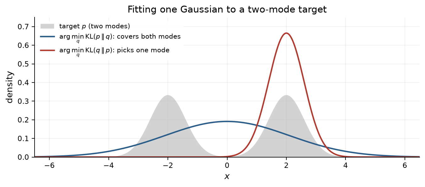
This trade-off only bites when the model can’t represent the data exactly, like the single Gaussian in Figure 4; with enough capacity, both directions have the same answer, \(P_\theta = P_{\text{data}}\). Sander Dieleman has a great practitioner’s take on it in his post on audio generation [13]. Likelihood-based models tend to be mode-covering, adversarial models tend to be mode-seeking, and which one you want depends on the task. Mode-covering buys diversity when the conditioning leaves a lot open, and mode-seeking buys realism when the conditioning already pins down most of the output, as in text-to-speech.
2.4 Data processing: you can’t create information
The most important property of \(f\)-divergences, alongside nonnegativity, is the data processing inequality (DPI). Take any “channel” \(P_{Y|X}\) that turns an input \(X\) into an output \(Y\). This could be a deterministic function, a noisy measurement, or a neural network encoder. If we feed it inputs from \(P_X\) and from \(Q_X\), we get outputs from \(P_Y\) and \(Q_Y\), and [9]
No processing can make two distributions easier to tell apart. The proof is Jensen again: the likelihood ratio of the outputs is a conditional expectation of the likelihood ratio of the inputs, and conditional expectation can only reduce the average of a convex function.
For machine learning, this means an encoder can throw information away, but it can never create it. For example, if you compare real and generated images through some feature extractor, any \(f\)-divergence between the feature distributions is at most the divergence between the images themselves.
A special case gets used over and over. Processing \(X\) into the indicator \(\mathbf{1}\{X \in A\}\) turns both distributions into Bernoulli distributions, so
for every event \(A\). A question about two whole distributions becomes a question about two numbers. This is the key step behind Pinsker’s inequality in Section 4.1.
2.5 Joint convexity: mixing makes things harder to distinguish
\(D_f(P\|Q)\) is convex in the pair \((P, Q)\) jointly [9]:
My favorite proof uses the DPI. Let a coin \(X \sim \mathrm{Ber}(\lambda)\) pick which pair we draw from, and let \(Y \sim P_X\) or \(Y \sim Q_X\). The divergence between the joint distributions of \((X, Y)\) is exactly the weighted average on the right, and forgetting \(X\) is a form of processing that turns them into the mixtures on the left. Intuitively, mixing hides which component a sample came from, so the mixtures are harder to tell apart.
The convexity is never strict, though. For example, \(\mathrm{TV}(\mathrm{Ber}(p), \mathrm{Ber}(q)) = |p - q|\) is piecewise linear. And convexity in each argument separately is the reason naive estimators of divergences are biased, which we’ll get to in Section 6.1.
3. Divergences as limits on classification
So far, divergences have been formal definitions. This section is the one that made them feel real to me: they measure exactly how well two hypotheses can be told apart from data.
3.1 Total variation and the best possible test
Suppose we observe \(X\) and know it comes from one of two known distributions, \(H_0 : X \sim P\) or \(H_1 : X \sim Q\). A test \(\varphi(x) \in \{0, 1\}\) decides which one. It can make two kinds of error: \(\alpha = P[\varphi(X) = 1]\) (rejecting a true \(H_0\)) and \(\beta = Q[\varphi(X) = 0]\) (accepting a false \(H_0\)). The Neyman–Pearson lemma says that optimal tests only ever look at the data through the likelihood ratio \(p(x)/q(x)\), thresholding it [14].
What’s the smallest possible \(\alpha + \beta\)? Write
The last integral is smallest if we reject exactly where it’s negative, i.e., where \(q(x) > p(x)\). Plugging that in:
where the last step uses the fact that \(p - q\) integrates to zero, so its positive and negative parts each carry half of \(\int |p - q|\) [9].
Total variation measures exactly how much better than a coin flip the best possible test is. If \(\mathrm{TV} = 0\), the best you can do is guess; if \(\mathrm{TV} = 1\), you never make a mistake. In classifier language, the best achievable balanced accuracy for telling samples of \(P\) from samples of \(Q\) is \(\tfrac12 (1 + \mathrm{TV}(P, Q))\). The DPI for TV becomes obvious from this angle too: if processing the data could help, the optimal test on the raw data wouldn’t have been optimal.
3.2 Bayes risk
The sum \(\alpha + \beta\) implicitly assumes both hypotheses are equally likely and both errors are equally costly. With prior probabilities \(\pi_0\) and \(\pi_1 = 1 - \pi_0\), the smallest weighted error is the Bayes risk [14]
the area under the lower of the two weighted densities (left panel of Figure 5). Pulling \(q(x)\) out of the minimum gives \(\int q\, f_\pi(p/q)\) with \(f_\pi(t) = \min\{\pi_0 t, \pi_1\}\). That function is concave, not convex, and \(f_\pi(1) \neq 0\), but \(h_\pi(t) = f_\pi(1) - f_\pi(t)\) fixes both problems (right panel of Figure 5). So \(D_{h_\pi}(P\|Q) = f_\pi(1) - R_\pi(P, Q)\): every Bayes risk is an \(f\)-divergence, up to a sign and a constant.
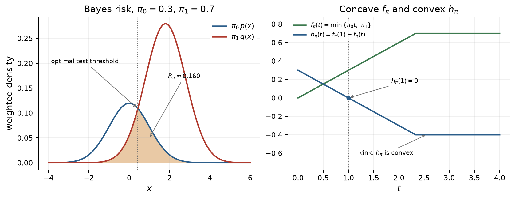
The converse is the surprising part. Call the statistical information at a prior \(\pi\) the amount by which observing \(X\) lowers the Bayes risk, compared with guessing from the prior alone. Every \(f\)-divergence can be written as an integral of this statistical information over all priors, weighted by a nonnegative function determined by the second derivative of \(f\) [14]. So choosing \(f\) means choosing which trade-offs between the two kinds of error you care about. Total variation puts all its weight on the balanced prior \(\pi_0 = \pi_1\), while KL spreads it over all priors.
This is also why “train a classifier to tell real from fake samples” and “measure a divergence between distributions” keep turning out to be the same thing in ML. We’ll make that precise in Section 6.3.
4. Inequalities between divergences
Why would anyone care how divergences relate to each other? Because one divergence is often easy to compute while another is easy to interpret. KL adds up over independent samples and has closed forms for Gaussians; TV is an error probability. Inequalities let you compute one and conclude something about the other.
The comparisons can’t be symmetric. TV and \(H^2\) are bounded, while KL and \(\chi^2\) can be infinite, so bounded divergences can always be controlled by unbounded ones, but not the other way around without extra assumptions.
4.1 Pinsker’s inequality
The most famous one bounds total variation by KL [15]:
and the constant is the best possible. I like the proof because it combines two tools from Section 2: the DPI from Section 2.4 and the event form of TV from Section 2.2.3.
- Reduce to two points. For any event \(A\), the DPI with the indicator of \(A\) gives \(\mathrm{KL}(P\|Q) \ge \mathrm{KL}(P(A)\,\|\,Q(A))\), where \(\mathrm{KL}(p\|q)\) is shorthand for the KL divergence between \(\mathrm{Ber}(p)\) and \(\mathrm{Ber}(q)\). If the inequality holds for Bernoulli distributions, then \(\sqrt{\mathrm{KL}(P\|Q)/2} \ge |P(A) - Q(A)|\) for every \(A\), and taking the supremum over \(A\) gives TV.
-
Prove it for Bernoullis. Using Taylor’s formula with integral remainder, and \(t(1-t) \le \tfrac14\),
\[ \mathrm{KL}(p\|q) = \int_q^p \frac{p - t}{t(1-t)}\, dt \ge 4 \int_q^p (p - t)\, dt = 2(p - q)^2. \]Since \(\mathrm{TV}(\mathrm{Ber}(p), \mathrm{Ber}(q)) = |p - q|\), we’re done [9].
In practice, Pinsker means small KL implies small TV, so convergence in KL, which is usually easier to prove, transfers to TV, which has an operational meaning. It shows up in RL theory too: the monotonic improvement bound behind TRPO is stated in terms of total variation and converted to KL with a Pinsker-type inequality [16].
The reverse direction fails in general. If \(P\) puts a little mass where \(q = 0\), TV is small but KL is infinite. On a finite alphabet where \(Q\) gives every outcome probability at least \(Q_{\min}\), a short computation gives \(\chi^2(P\|Q) \le 2\,\mathrm{TV}^2 / Q_{\min}\) and therefore
The constant blows up as \(Q_{\min} \to 0\), exactly as the counterexample predicts [15].
4.2 Hellinger, TV and χ²
For the bounded divergences, comparisons work in both directions [9]:
The proof is two lines. The left side follows by integrating
For the right side, write \(|p - q| = |\sqrt p - \sqrt q| \cdot (\sqrt p + \sqrt q)\) and apply Cauchy–Schwarz, using \(\int (\sqrt p + \sqrt q)^2 = 4 - H^2\).
So TV and Hellinger go to zero together and reach their maxima together, although not at the same speed. Combined with the product rule for Hellinger from Section 2.2.4, this is why Hellinger is the standard tool for asking whether two families of hypotheses can be told apart asymptotically.
Cauchy–Schwarz also gives \(\mathrm{TV} \le \tfrac12\sqrt{\chi^2}\), and together with \(H^2 \le \mathrm{KL} \le \log(1 + \chi^2) \le \chi^2\) we get a hierarchy in which \(\chi^2\) controls everything else. A theorem by Harremoës and Vajda explains why reductions to Bernoulli distributions keep giving the best constants: the boundary of the set of all achievable pairs \((D_f(P\|Q), D_g(P\|Q))\) is always attained by distributions on just two points [9].
4.3 Le Cam’s two-point method: where 1/√n comes from
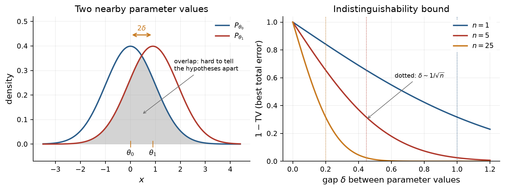
These inequalities are the workhorse behind lower bounds in estimation theory. Le Cam’s idea is to pick just two parameter values \(\theta_0\) and \(\theta_1\) that are far apart, but whose data distributions are close. No estimator can be accurate for both, because an accurate estimator would give a good test between them, and Section 3.1 limits how good any test can be [9].
For \(n\) i.i.d. samples, total variation between the product distributions is hard to compute, but KL simply adds up: \(\mathrm{KL}(P^n\|Q^n) = n\,\mathrm{KL}(P\|Q)\). For the mean of a Gaussian, with \(\theta_1 - \theta_0 = 2\delta\), Pinsker gives
So as long as \(\delta\) is much smaller than \(1/\sqrt n\) (written \(\delta \ll 1/\sqrt n\)), the total variation is close to zero, and by Section 3.1 no test can do much better than a coin flip: the two hypotheses are practically indistinguishable. Figure 6 shows this for several sample sizes. That’s the information-theoretic reason why estimation error in regular parametric models scales like \(1/\sqrt n\).
5. Zooming in: local behavior and Fisher information
In statistics and ML, we usually compare nearby members of a parametric family \(\{P_\theta\}\), not two arbitrary distributions. What does \(D_f(P_t\|P_0)\) look like when \(t\) is small?
5.1 Every smooth \(f\)-divergence is χ² up close
Write the likelihood ratio as \(p_t / p_0 = 1 + \varepsilon_t\), where \(\varepsilon_t \to 0\), and expand \(f\) around \(1\):
The linear term integrates to zero, for the same reason adding \(c(t-1)\) to \(f\) changes nothing (Section 2.1). What’s left is
Locally, every smooth \(f\)-divergence is \(\chi^2\) in disguise, and the choice of \(f\) only affects the constant \(f''(1)/2\) [9].
5.2 Fisher information
For a smooth family, \(\chi^2(P_t\|P_0)/t^2\) converges to
the Fisher information. Putting it together, for a multi-parameter family,
| Divergence | \(f''(1)\) | Local behavior |
|---|---|---|
| \(\chi^2\) | \(2\) | \(J_F\, t^2\) |
| KL | \(1\) | \(\tfrac12 J_F\, t^2\) |
| \(H^2\) | \(\tfrac12\) | \(\tfrac14 J_F\, t^2\) |
| JS | \(\tfrac12\) | \(\tfrac14 J_F\, t^2\) |
| TV | — | linear in \(\lvert t \rvert\), not \(t^2\) |
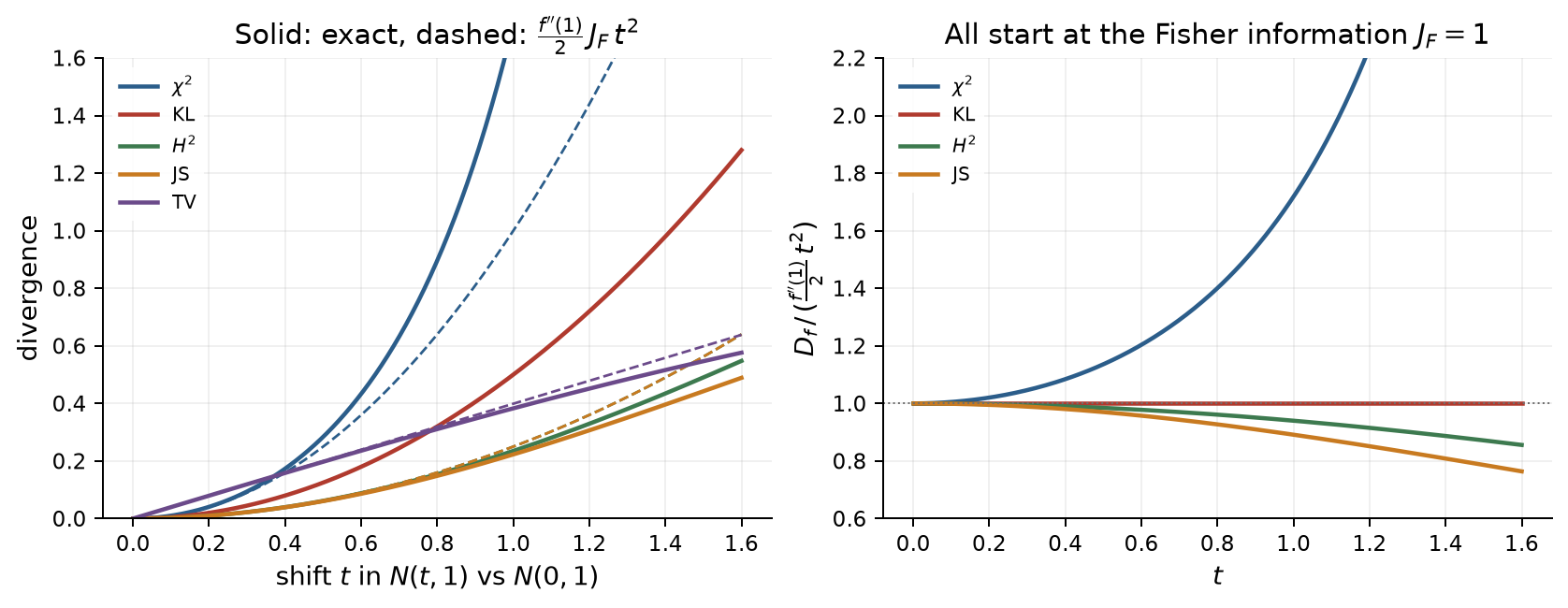
Total variation is the exception again. Its generator isn’t differentiable at \(1\), and it grows linearly: for \(P_t = N(t, 1)\), \(\mathrm{TV}(P_t, P_0) \approx |t|/\sqrt{2\pi}\).
Figure 7 checks all of this on the family \(N(t, 1)\), whose Fisher information is \(J_F = 1\). In the right panel, each divergence is divided by its predicted quadratic \(\tfrac{f''(1)}{2} t^2\), so the local result says every curve should start at \(1\), and they all do. Away from \(t = 0\), though, the quadratic approximation is no longer exact, and each divergence drifts off in its own way:
- KL stays flat at \(1\), because for two Gaussians with the same variance it’s exactly \(t^2/2\).
- Hellinger and JS bend down. They’re bounded (by \(2\) and \(2\log 2\)), so they must eventually fall below any parabola.
- \(\chi^2\) shoots up. For these Gaussians it equals \(e^{t^2} - 1 = t^2 + t^4/2 + \dots\), which grows much faster than \(t^2\). This is the variance-of-the-likelihood-ratio view from Section 2.2.2 at work: squaring the ratio \(p/q\) makes \(\chi^2\) dominated by the tails, where \(q\) is tiny and the ratio is huge.
5.3 What this means for ML
Geometrically, all smooth \(f\)-divergences induce the same local quadratic form, and the Fisher information is the metric tensor that information geometry is built on. This has very practical consequences:
- Natural gradient [17]. Instead of taking the steepest step in parameter space, take the steepest step among parameters at a fixed KL distance. Since that KL is locally \(\tfrac12 h^\top J_F h\), the update becomes \(h \propto -J_F^{-1} \nabla L\), which doesn’t depend on how you parameterize the model.
- Trust regions in RL. TRPO constrains the KL divergence between the old and the new policy, and solves the constrained problem using exactly this quadratic Fisher approximation [16]. PPO’s clipping is a cheaper proxy for the same idea [18].
- For small steps, the choice of divergence barely matters. Every smooth \(f\)-divergence is approximately \(\tfrac{f''(1)}{2}\, h^\top J_F h\), so KL, \(\chi^2\) and Hellinger trust regions agree up to a constant factor, and two divergences with the same \(f''(1)\) agree completely, up to higher-order terms. Differences only show up for large steps. This is exactly why the \(k_2\) estimator of KL in Section 6.5.2 has such a small bias.
6. Estimating divergences from samples
Everything so far assumed we know \(P\) and \(Q\). In practice we only have samples \(X_1, \dots, X_n \sim P\) and \(Y_1, \dots, Y_m \sim Q\). Estimating a divergence is much harder than estimating a mean, because \(D_f\) depends on the distributions nonlinearly, through their ratio, so it’s not the expectation of any known function of the data [19].
6.1 Why plug-in estimates are bad
The obvious approach for discrete data with \(k\) possible outcomes is to replace the distributions by empirical frequencies \(\hat p_i = N_i / n\) and compute \(D_f(\hat p\|\hat q)\). This is consistent when \(k\) is fixed and \(n \to \infty\), but it’s systematically biased upward. Even with \(Q\) known, convexity (Section 2.5) and Jensen give
If \(P = Q\), the true value is zero, but the estimate is positive unless the sample frequencies happen to match \(Q\) exactly.
Section 5 even tells us how big the bias is. The error \(\hat p - p\) is of order \(1/\sqrt n\), the divergence is locally quadratic with constant \(f''(1)/2\), and \(\mathbb{E}[\chi^2(\hat p\|p)] = (k-1)/n\), so, at least when \(P\) and \(Q\) are close [9],
For KL, that’s about \((k-1)/(2n)\), and in that case it holds for any \(Q\). The bias depends on the number of outcomes \(k\), not just the sample size. When \(k\) is comparable to \(n\) or larger, the bias is as large as the quantity being estimated. Think of distributions over a language model’s vocabulary, where \(k\) is in the hundreds of thousands. For continuous data it’s even worse: the empirical distribution has no density, so the plug-in estimate isn’t defined without first estimating densities, which runs into the curse of dimensionality.
The key observation is that \(D_f(P\|Q)\) doesn’t need \(p\) and \(q\) separately, only their ratio \(p/q\). That’s a single function, and it’s often much smoother than either density. The question is how to estimate it without estimating the densities.
6.2 The variational representation
The answer is convex duality. The convex conjugate of \(f\) is \(f^*(v) = \sup_u \{uv - f(u)\}\), and for convex \(f\) the relation goes both ways: \(f(u) = \sup_v \{uv - f^*(v)\}\). Plugging this into the definition, pointwise at \(u = p(x)/q(x)\), and swapping the supremum with the integral gives [19]
with the supremum attained at \(g^* = f'(p/q)\). Restricting \(g\) to any smaller class gives a lower bound.
This is the most useful formula in the post for ML. There are no densities in it, only two expectations, one under \(P\) and one under \(Q\). Replace them with sample averages, let \(g\) be a neural network (a “critic”), and maximize with SGD. As a bonus, the optimal critic is a transformed likelihood ratio, so you get an estimate of \(p/q\) for free.
For KL, \(f^*(v) = e^{v-1}\), which gives \(\mathrm{KL}(P\|Q) = \sup_g \{\mathbb{E}_P[g] - \mathbb{E}_Q[e^{g-1}]\}\) with optimum \(g = 1 + \log(p/q)\) [19]. A closely related and tighter form is the Donsker–Varadhan representation, \(\mathrm{KL}(P\|Q) = \sup_g \{\mathbb{E}_P[g] - \log \mathbb{E}_Q[e^{g}]\}\), which MINE uses to estimate mutual information with neural networks [20]. For total variation, \(f\) isn’t differentiable, and the optimal \(g\) only tells you where \(p > q\), not by how much. That’s just the optimal test from Section 3.1.
6.3 Every classifier is a density ratio estimator
There’s an even more direct way to get the ratio. Train a probabilistic classifier \(D(x)\) to distinguish samples of \(P\) (label 1) from samples of \(Q\) (label 0), with balanced classes and the usual logistic loss. The optimal classifier is \(D^*(x) = p(x) / (p(x) + q(x))\), so
So every classifier you train to tell two datasets apart is secretly a density ratio estimator, and through the formula in Section 6.2, a divergence estimator. A GAN discriminator is exactly this. f-GAN [21] makes the connection explicit: pick any \(f\), use the variational bound as the GAN objective, and the original GAN falls out as the Jensen–Shannon case.
6.4 Mutual information
Mutual information is also an \(f\)-divergence: \(I(X; Y) = \mathrm{KL}(P_{XY}\|P_X \otimes P_Y)\), the KL divergence between the joint distribution and the product of the marginals. Both are easy to sample from a single dataset of pairs \((X_i, Y_i)\): the pairs themselves are samples from \(P_{XY}\), and shuffling the \(Y\)’s gives (approximately) samples from \(P_X \otimes P_Y\). Plugging these into a variational bound gives neural MI estimators like MINE [20]. The InfoNCE objective behind contrastive learning [22] is a related lower bound on mutual information. It has low variance, but it can never exceed the log of the batch size [23].
6.5 Estimating the KL penalty in RLHF
This part wasn’t in my paper, but it’s where these ideas finally clicked for me. When a language model is fine-tuned with RL, the objective usually includes a penalty \(\beta \cdot \mathrm{KL}(\pi_\theta\|\pi_{\text{ref}})\) that keeps the policy \(\pi_\theta\) close to a reference model \(\pi_{\text{ref}}\), typically the supervised fine-tuned starting point [6], [7]. This prevents the policy from drifting into degenerate text that happens to fool the reward.
This setting is different from Sections 6.1–6.4. Both models give us log-probabilities, so we can compute the likelihood ratio exactly for any token, and there’s nothing to learn. The only problem is that the KL is an average over all possible sequences, far too many to sum over, so in practice it’s estimated from the tokens the policy actually sampled. For a sampled token \(x \sim \pi_\theta\), let \(r = \pi_{\text{ref}}(x) / \pi_\theta(x)\). We want \(\mathrm{KL}(\pi_\theta\|\pi_{\text{ref}}) = \mathbb{E}_{\pi_\theta}[-\log r]\). John Schulman’s blog post [24] compares three per-sample estimators. Each is computed from a single sampled token, and averaging it over many samples estimates the KL.
6.5.1 \(k_1 = -\log r\): unbiased but noisy
This is the direct estimator. Its average is exactly the KL, so it’s unbiased. But it has high variance, and it’s negative whenever the reference likes a token more than the policy does (\(r > 1\)), even though the KL itself is never negative.
6.5.2 \(k_2 = \tfrac12 (\log r)^2\): low variance, slightly biased
This one is never negative and has low variance, but it’s biased: its average isn’t exactly the KL. The bias is small as long as the policy stays close to the reference, and Section 5 explains why:
- The average of \(k_2\) is itself an \(f\)-divergence: \(\mathbb{E}_{\pi_\theta}[k_2] = D_{f_2}(\pi_{\text{ref}}\|\pi_\theta)\) with \(f_2(t) = \tfrac12 (\log t)^2\).
- The KL we want is also an \(f\)-divergence: \(\mathrm{KL}(\pi_\theta\|\pi_{\text{ref}}) = D_{f}(\pi_{\text{ref}}\|\pi_\theta)\) with \(f(t) = -\log t\).
- Both generators have the same second derivative at \(1\): \(f_2''(1) = f''(1) = 1\). So by Section 5.2, when the policy is a small step \(h\) away from the reference, both divergences are approximately \(\tfrac12\, h^\top J_F h\), the same Fisher-information quadratic.
The two only differ in higher-order terms, which is why \(k_2\) is nearly unbiased near the reference, and why its bias grows once the policy drifts away.
6.5.3 \(k_3 = (r - 1) - \log r\): unbiased and low variance
This one gets the best of both. It’s unbiased because
so adding \(r - 1\) to \(k_1\) doesn’t change its average. It does cancel much of its noise, though: when \(k_1 = -\log r\) is very negative (\(r\) large), \(r - 1\) is very positive. That’s exactly the “add \(c(t-1)\) to \(f\)” freedom from Section 2.1. And \(k_3\) is never negative, because the convex function \(-\log r\) lies above its tangent line at \(r = 1\), which is \(1 - r\), and \(k_3\) is exactly the vertical gap between the two. (A gap like this, between a convex function and its tangent line, is called a Bregman divergence.)
6.5.4 How they compare
Figure 8 shows the difference. On the left, all three estimators are zero at \(r = 1\), but only \(k_1\) dips below zero. On the right are single-sample estimates for a toy policy and reference: all three have the right average (up to \(k_2\)’s small bias), but \(k_1\) is spread over a wide range of positive and negative values, while \(k_2\) and \(k_3\) are never negative and much more concentrated.
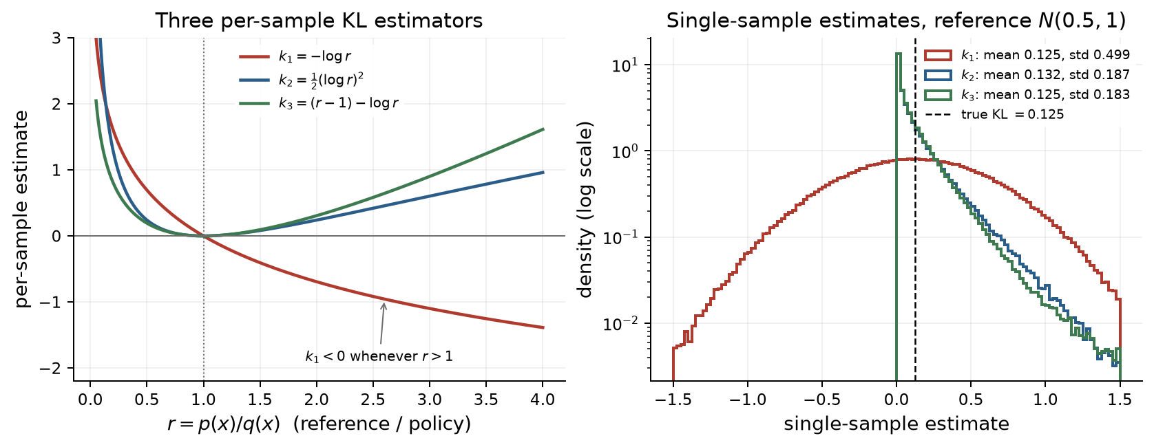
To check the numbers, I reran Schulman’s Gaussian experiment: policy \(N(0,1)\), reference \(N(\mu, 1)\), true KL \(\mu^2/2\). The table shows the bias and the standard deviation of a single-sample estimate, both relative to the true KL. Bias is given as a percentage of the KL. Standard deviation is given as a multiple of it, so a value of \(20\) means one sample’s noise is 20 times the quantity you’re estimating (averaging \(N\) samples divides it by \(\sqrt N\)).
| Reference | True KL | \(k_1\) bias | \(k_1\) std | \(k_2\) bias | \(k_2\) std | \(k_3\) bias | \(k_3\) std |
|---|---|---|---|---|---|---|---|
| \(N(0.1, 1)\) | \(0.005\) | \(0\%\) | \(20\) | \(0.25\%\) | \(1.42\) | \(0\%\) | \(1.42\) |
| \(N(0.5, 1)\) | \(0.125\) | \(0\%\) | \(4.0\) | \(6.25\%\) | \(1.50\) | \(0\%\) | \(1.48\) |
| \(N(1, 1)\) | \(0.5\) | \(0\%\) | \(2.0\) | \(25\%\) | \(1.73\) | \(0\%\) | \(1.70\) |
These values agree with a two-million-sample simulation and with exact formulas for this Gaussian case: \(k_1\) has relative standard deviation \(2/\mu\); \(k_2\) has relative bias \(\mu^2/4\) and relative standard deviation \(\sqrt{2 + \mu^2}\); and \(k_3\) has relative standard deviation \(\sqrt{e^{\mu^2} - 1 - \mu^2}\,/\,(\mu^2/2)\). Close to the reference (first row), \(k_1\)’s noise is 20 times the signal, while \(k_2\) and \(k_3\) are practically identical. Further away, \(k_2\)’s bias grows to 25%, and \(k_3\) stays unbiased with the lowest variance of the three.
6.5.5 What TRL does
The GRPO algorithm from DeepSeekMath uses \(k_3\) as its KL term [25], and Hugging Face’s TRL library
implements it exactly that way. This is the per-token KL in GRPOTrainer [26], where
ref_per_token_logps - per_token_logps is \(\log r\):
per_token_kl = (
    torch.exp(ref_per_token_logps - per_token_logps) - (ref_per_token_logps - per_token_logps) - 1
)
That’s \(e^{\log r} - \log r - 1 = (r - 1) - \log r\), which is \(k_3\).
TRL’s RLOOTrainer makes a different choice: it uses \(k_1\) (old_per_token_logps - ref_per_token_logps), sums it over
all the tokens of a sequence, and subtracts it from the reward instead of adding it to the loss [26]. A comment
in the TRL source says this is intentional and follows the RLOO paper [27], which in turn follows the
original RLHF setup [6]. My reading of why it makes sense: the KL-regularized objective can be written as
a single expectation,
and the log-ratio of a whole sequence \(y\) is exactly \(k_1\) summed over its tokens. So putting \(k_1\) into the reward makes a REINFORCE-style method like RLOO optimize precisely the regularized objective. Negative per-token values don’t matter there, because they’re just summed into one scalar reward per sequence. GRPO instead adds the KL to the loss token by token, where a nonnegative, low-variance per-token estimate like \(k_3\) is the natural choice.
One last connection: the penalty is the reverse KL from the policy’s point of view, which by Section 2.3 means it’s mode-seeking. It punishes the policy for producing text the reference finds unlikely, but it doesn’t stop the policy from dropping some of the reference’s modes. That’s one explanation offered for the loss of output diversity after RL fine-tuning.
7. Where \(f\)-divergences break: Wasserstein distance
All \(f\)-divergences share one structural limitation, and it comes straight from the definition. They compare the densities \(p(x)\) and \(q(x)\) at the same point \(x\). The geometry of the space, meaning how far apart two points are, never enters the formula.
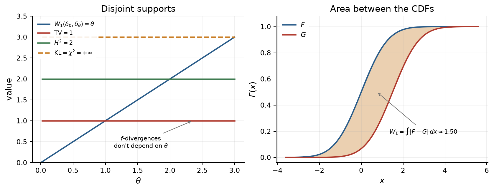
The simplest example makes this painfully clear. Let \(P = \delta_0\) and \(Q_\theta = \delta_\theta\) be point masses at \(0\) and \(\theta\). For every \(\theta \neq 0\), the supports are disjoint, so
no matter what \(\theta\) is. For \(\theta = 0.01\) and for \(\theta = 100\), every \(f\)-divergence gives the same answer, even though in the first case the distributions are practically identical.
This isn’t just a curiosity. If you train a model \(Q_\theta\) by minimizing an \(f\)-divergence to the data, and their supports don’t overlap, the divergence is constant in \(\theta\), the gradient is zero, and optimization can’t make any progress. Real data like images concentrates near low-dimensional manifolds, and two such manifolds in a high-dimensional space almost never overlap. Arjovsky and Bottou showed that this is the root of the vanishing gradient problem in the original GAN, where Jensen–Shannon simply saturates [4].
This is also one reason generative models add noise. Arjovsky and Bottou suggested adding noise to both distributions so that their supports overlap [4]. Score-based diffusion models perturb the data with Gaussian noise partly for the same reason: data on a low-dimensional manifold doesn’t even have a well-defined score (the gradient of its log-density), while the noisy distribution covers the whole space [28]. And normalizing flows add small uniform noise to discrete pixel values, called dequantization, so that a continuous density can’t cheat by putting infinite density on the discrete values [29].
7.1 Moving mass: Wasserstein distance
What we need is a different question. Instead of “how different are the two densities at each point?”, ask “how much work does it take to turn one distribution into the other?” Think of \(P\) as a pile of dirt and \(Q\) as the shape you want to build. Moving a bit of dirt costs its amount times the distance it travels, and the distance between the distributions is the cheapest total cost of the whole job. This is the oldest question in optimal transport: Gaspard Monge posed it in 1781, literally about how to move soil from excavations to embankments [30]. That’s also why the resulting distance is known in computer science as the earth mover’s distance [31]. Figure 9 illustrates the idea.
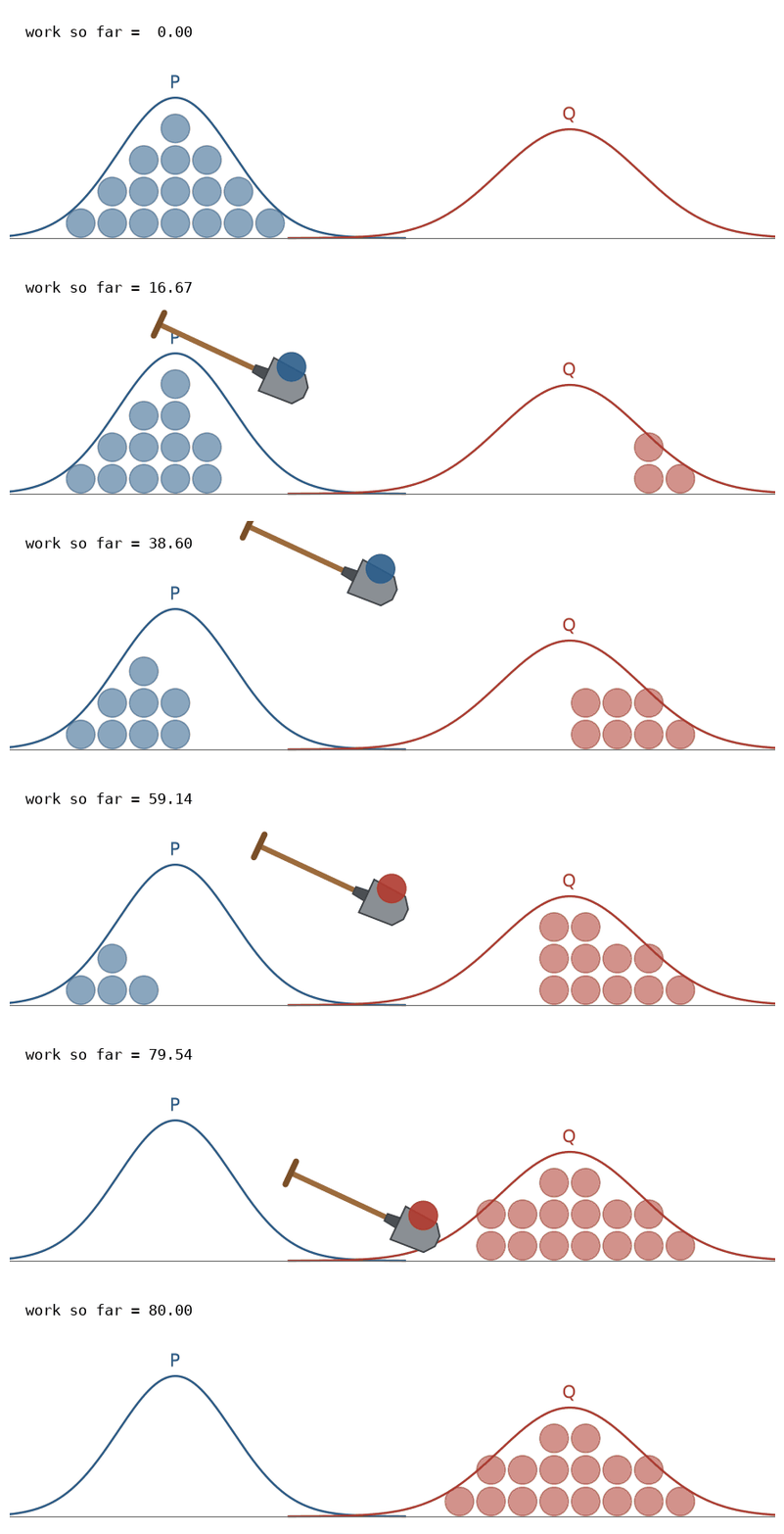
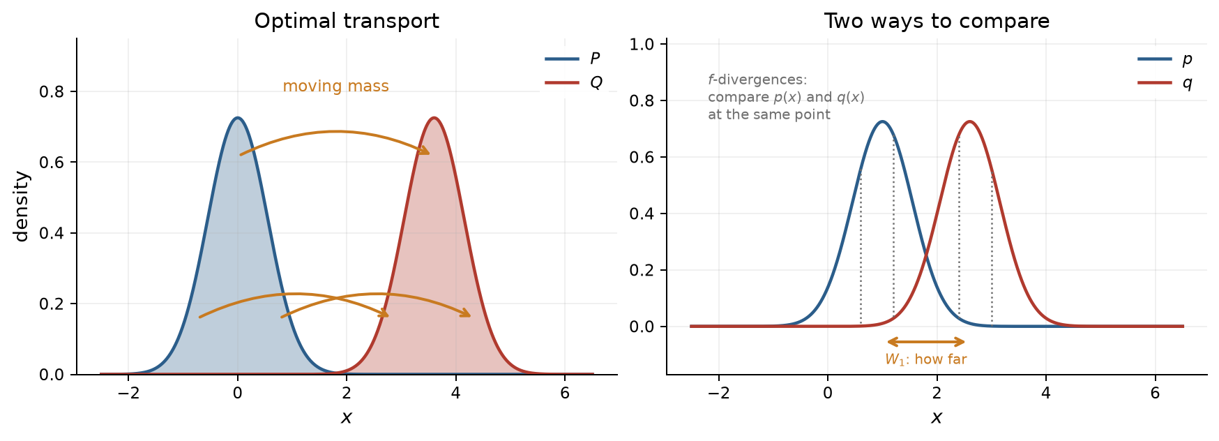
Figure 10 shows the contrast with \(f\)-divergences on a one-dimensional example. \(f\)-divergences compare the two densities vertically, point by point, while optimal transport asks how far mass has to travel horizontally. The picture is one-dimensional to keep it simple, but the same idea works in any number of dimensions.
Formally, the Wasserstein distance of order \(p \ge 1\) is [32]
where \(\Gamma(P, Q)\) is the set of couplings: joint distributions whose marginals are \(P\) and \(Q\). Each coupling is a transport plan, where \(\gamma(x, y)\) says how much of the mass at \(x\) is moved to \(y\), and \(\|x - y\|^p\) is the cost of moving it. The points \(x\) and \(y\) can live in any number of dimensions, and \(\|x - y\|\) is the usual Euclidean distance between them.
Note that \(p\) is the order, not the dimension: it’s the power the distance is raised to in the cost. \(W_1\) charges amount times distance, like the dirt-moving picture, while \(W_2\) charges amount times distance squared, which makes long moves disproportionately expensive. Both show up in ML: \(W_1\) in Wasserstein GANs (Section 7.2) and \(W_2\) in flow matching (Section 7.4).
For the point masses from the start of this section, there’s only one plan, moving everything from \(0\) to \(\theta\), so \(W_p(\delta_0, \delta_\theta) = |\theta|\). It grows with the distance, exactly as intuition demands, even though the supports never overlap. The left panel of Figure 11 shows it next to the saturated \(f\)-divergences.
Two more properties make \(W_p\) attractive. First, unlike KL, it’s a true metric: symmetric, and it satisfies the triangle inequality. Second, it can see distributions converge even when their supports never overlap. Take \(P_n = \delta_{1/n}\), a point mass that slides toward \(0\). For every \(n\), \(\mathrm{TV}(P_n, \delta_0) = 1\) and \(\mathrm{KL} = \infty\), so no \(f\)-divergence notices that \(P_n\) is getting closer to \(\delta_0\), but \(W_p(P_n, \delta_0) = 1/n \to 0\). In technical terms, convergence in \(W_p\) is equivalent to weak convergence (averages of every bounded continuous function converge) plus convergence of the \(p\)-th moments, which keeps mass from escaping to infinity [32].
7.2 Kantorovich duality
Computing \(W_p\) means solving an optimization problem over couplings, so a dual form is extremely useful. For any order \(p\), with \(x\) and \(y\) in any number of dimensions, Kantorovich duality says [30]
There’s a nice economic reading of this. Imagine a shipping company that charges \(\varphi(x)\) to pick up a unit of dirt at \(x\) and \(\psi(y)\) to drop it off at \(y\). To stay competitive, its combined price can never exceed what it would cost you to move the dirt yourself, \(\|x - y\|^p\). The most it can earn under that rule is exactly the optimal transport cost.
For \(p = 1\), the two price functions collapse into one, and the constraint turns into a smoothness condition. A function \(g\) is 1-Lipschitz if
meaning its value can’t change faster than the distance between its inputs. For a differentiable function of one variable, that just says its slope is at most \(1\) in absolute value, \(|g'(x)| \le 1\); in several dimensions, it says the gradient has norm at most \(1\). (More generally, \(g\) is \(L\)-Lipschitz if \(|g(x) - g(y)| \le L\,\|x - y\|\).) With that, the optimal \(\psi\) is simply \(-\varphi\), and we get the Kantorovich–Rubinstein duality [32]:
Compare this with the variational formula for \(f\)-divergences from Section 6.2. Both are “the supremum, over critics \(g\), of a difference of two expectations”. For \(f\)-divergences, \(g\) can be anything, but the second term goes through \(f^*\). For \(W_1\), the second term is plain, but \(g\) has to be 1-Lipschitz. That constraint is exactly where geometry enters: nearby points must get nearby values. This is the idea behind the Wasserstein GAN, whose critic is kept Lipschitz, first by weight clipping [5] and later with a gradient penalty that pushes the norm of the critic’s gradient toward \(1\) [33].
The two families are comparable in only one direction. On a space with diameter \(\mathrm{diam}\), we have \(W_1 \le \mathrm{diam} \cdot \mathrm{TV}\), because no mass travels further than the diameter, but the point-mass example shows there’s no reverse bound. Wasserstein distance is a weaker measure of difference, and that weakness is exactly what makes it give useful gradients when \(f\)-divergences give none.
7.3 One dimension: sort and match
In one dimension, optimal transport has a completely explicit solution. Mass is moved monotonically: the smallest values of \(P\) go to the smallest values of \(Q\), and so on, so transport paths never cross. This is also the plan the shovel follows in Figure 9. With CDFs \(F\) and \(G\) and quantile functions \(F^{-1}\) and \(G^{-1}\) [32],
and the optimal map is \(T = G^{-1} \circ F\). For \(p = 1\), it gets even better:
Both integrals measure the same area between the two CDFs, once horizontally and once vertically (right panel of Figure 11). This closes the loop with Section 1: the Kolmogorov–Smirnov statistic is the supremum of \(|F_n - F_0|\), and \(W_1\) is its integral version. Both compare CDFs, which is why neither is an \(f\)-divergence. For two samples of the same size, you don’t need any density estimation at all: sort both samples and pair them up, \(W_p(P_n, Q_n) = \big( \tfrac1n \sum_i |X_{(i)} - Y_{(i)}|^p \big)^{1/p}\).
The two ways of comparing distributions also give two different “straight lines” from \(P\) to \(Q\), shown in Figure 12:
- The mixture path \((1-t)P + tQ\) fades mass out in one place and fades it in somewhere else. It’s the straight line for total variation, the simplest \(f\)-divergence: since \((1-t)P + tQ - P = t(Q - P)\), we get \(\mathrm{TV}(P, (1-t)P + tQ) = t \cdot \mathrm{TV}(P, Q)\), so TV grows at a constant speed along it. Measured by \(W_2\), though, it rushes ahead early.
- The transport path slides every quantile along a straight line, \(x_t = (1-t)\,x + t\,T(x)\). It’s the straight line for \(W_2\), with \(W_2(P, \rho_t) = t \cdot W_2(P, Q)\). Measured by TV, though, it almost jumps: as soon as the moving mass stops overlapping with \(P\), TV is nearly \(1\), even though the mass has barely moved.
Two details are worth spelling out. First, why \(W_2\) and not \(W_1\)? Because \(W_1\) can’t tell these two paths apart. Picture \(P\) and \(Q\) as two lumps of mass a distance \(d\) apart. At time \(t\), the mixture path has moved a fraction \(t\) of the mass the whole distance \(d\), while the transport path has moved all of the mass a distance \(td\). \(W_1\) charges mass times distance, so both cost \(t \cdot d\), and both paths move at a constant speed in \(W_1\). (In general, \(W_1(P, (1-t)P + tQ) = t \cdot W_1(P, Q)\), because the Kantorovich–Rubinstein formula only depends on \(P - Q\).) \(W_2\) charges mass times distance squared, which punishes long moves. The mixture path costs \(t \cdot d^2\), so \(W_2 = \sqrt t \cdot d\), while the transport path costs \(1 \cdot (td)^2\), so \(W_2 = t \cdot d\). Only the transport path moves at a constant speed, and \(\sqrt t\) is why the mixture path rushes ahead early in Figure 12. \(W_2\) is also the distance behind flow matching, where the squared distance becomes kinetic energy (Section 7.4).
Second, total variation stays finite along both paths, even once the moving mass no longer overlaps with \(P\); it just saturates, because it can never exceed \(1\). It equals \(1\) only when the two distributions share no mass at all. Gaussian densities are positive everywhere, so \(P\) and \(Q\) technically do overlap, but only where both are tiny: they share about \(0.03\%\) of their mass, so \(\mathrm{TV}(P, Q) \approx 0.9997\). The readouts in Figure 12 show TV as a percentage of this value.
The bottom path is the natural one for a flow model. An ODE moves mass continuously, so it can’t make mass disappear in one place and reappear in another. To follow the top path, it would have to rush mass through the almost empty gap between \(P\) and \(Q\) at enormous speed (infinite speed, if the supports were truly disjoint). That’s the bridge to the last subsection.
7.4 Why this matters for flow matching
Flow matching learns a velocity field \(v_t(x)\) and generates samples by solving the ODE \(\frac{d}{dt} x_t = v_t(x_t)\), which carries noise samples at \(t = 0\) to data samples at \(t = 1\) [1]. Its standard “conditional optimal transport” path moves each sample along a straight line. That isn’t an arbitrary choice, and the reason becomes clear once you see optimal transport as motion instead of a static plan.
Picture the mass of \(P\) flowing into \(Q\) over time \(t \in [0, 1]\). At each moment, \(\rho_t(x)\) is the density of the mass and \(v_t(x)\) is its velocity at the point \(x\), the same kind of object flow matching learns. Two ingredients describe such a flow:
- Mass is conserved. It isn’t created or destroyed; it only moves. This is the continuity equation, \(\partial_t \rho_t + \nabla \cdot (\rho_t v_t) = 0\): the density at a point changes only because mass flows in or out of it. It’s the formal version of “no teleporting” from Figure 12.
- Moving mass costs kinetic energy. The total cost of a flow is \(\int_0^1 \int \|v_t(x)\|^2 \rho_t(x)\, dx\, dt\): squared speed, weighted by how much mass moves at that speed, added up over time. It’s the \(\tfrac12 m v^2\) from physics, without the \(\tfrac12\).
The Benamou–Brenier formula [34] says that the cheapest flow from \(P\) to \(Q\) costs exactly \(W_2^2\):
In the cheapest flow, every particle moves in a straight line at constant speed, since any detour or change of speed wastes kinetic energy. That’s the transport path from Figure 12, and it’s why straight paths are the natural target for flow matching. The flow that flow matching actually learns from independently paired noise and data isn’t optimal in general, so its trajectories curve and need more ODE steps to integrate. Rectified flow [35] and minibatch optimal transport couplings [8], [36] are ways of straightening them.
In one dimension, there’s a clean guarantee about the endpoints. ODE trajectories can’t cross, so the map from noise to data defined by any flow is increasing, and the only increasing map that pushes a continuous \(P\) onto \(Q\) is \(G^{-1} \circ F\) from Section 7.3, the optimal transport map. So in 1D, every flow model ends up with the optimal transport map between its endpoints, even though its trajectories in between needn’t be straight. In higher dimensions there’s no such guarantee, which is why the choice of coupling matters so much in flow matching. And optimal transport isn’t always what you want: with paired data, for example, you might want the flow to respect the given pairs rather than the cheapest ones.
8. Conclusion
The main thing I took away from this project is how much follows from one definition. An \(f\)-divergence compares two distributions through the likelihood ratio, and the convex function \(f\) only decides how deviations of that ratio are penalized. From there:
- Nonnegativity, the data processing inequality and joint convexity hold for every \(f\), with proofs that are basically Jensen’s inequality (Section 2).
- They have operational meaning. Total variation is exactly how well the best classifier can do, and every \(f\)-divergence is a weighted integral, over all priors, of how much the data lowers the Bayes risk (Section 3).
- Inequalities let you compute one divergence and conclude something about another. Pinsker and Le Cam’s method explain where the familiar \(1/\sqrt n\) comes from (Section 4).
- Locally, they’re all the same: every smooth \(f\)-divergence is \(f''(1)/2\) times the same Fisher-information quadratic (Section 5). That’s the geometry behind natural gradients and trust regions. It also explains why the \(k_2\) estimator is nearly unbiased near the reference: its average is an \(f\)-divergence with the same \(f''(1)\) as the KL it estimates (Section 6.5.2).
- Estimation from samples should go through the variational representation, which means through critics and classifiers, rather than through plugging in empirical frequencies (Sections 6.1–6.4). When both densities can be evaluated, as with language models, simple per-sample estimators work instead, and the best of them, \(k_3\), is a small, beautiful application of the freedom in choosing \(f\) (Section 6.5).
- Their limitation is structural. They compare densities point by point, so they’re blind to the geometry of the space (Section 7).
So when should you use which? My paper ended with a comparison between \(f\)-divergences and Wasserstein distance, and I still think it’s the right summary:
| \(f\)-divergences | Wasserstein distance | |
|---|---|---|
| What it compares | the densities, point by point, through \(p/q\) | how far mass has to move |
| Uses the geometry of the space | no | yes, through the distance between points |
| Disjoint supports | saturates (TV, \(H^2\), JS) or is infinite (KL, \(\chi^2\)) | stays finite and grows with the distance |
| Interpretation | information and testing: DPI, optimal error, likelihood | transport cost; a true metric |
| Computation | simple with densities; from samples via variational bounds | 1D: sort the samples; higher dimensions: OT solvers or Lipschitz critics |
| Best when | distributions share support, and distinguishability or information is what matters | supports may not overlap, or the geometry of the space matters |
In short: if the distributions live on the same support and you care about how distinguishable they are, \(f\)-divergences are the natural choice, with a precise meaning in terms of testing and information. If the supports might not overlap, which is typical for data on low-dimensional manifolds, or if the geometry of the space matters, Wasserstein distance is the better tool. The price is losing the information-theoretic interpretation and harder computation in high dimensions.
If you spot a mistake here, I’d be grateful if you let me know.
References
- Y. Lipman, R. T. Q. Chen, H. Ben-Hamu, M. Nickel, M. Le. Flow Matching for Generative Modeling. ICLR, 2023.
- C. M. Bishop. Pattern Recognition and Machine Learning, Sections 1.6.1 and 10.1.2. Springer, 2006.
- I. Goodfellow, J. Pouget-Abadie, M. Mirza, B. Xu, D. Warde-Farley, S. Ozair, A. Courville, Y. Bengio. Generative Adversarial Nets. NeurIPS, 2014.
- M. Arjovsky, L. Bottou. Towards Principled Methods for Training Generative Adversarial Networks. ICLR, 2017.
- M. Arjovsky, S. Chintala, L. Bottou. Wasserstein Generative Adversarial Networks. ICML, 2017.
- D. M. Ziegler, N. Stiennon, J. Wu, T. B. Brown, A. Radford, D. Amodei, P. Christiano, G. Irving. Fine-Tuning Language Models from Human Preferences. arXiv:1909.08593, 2019.
- L. Ouyang et al. Training Language Models to Follow Instructions with Human Feedback. NeurIPS, 2022.
- A. Tong, K. Fatras, N. Malkin, G. Huguet, Y. Zhang, J. Rector-Brooks, G. Wolf, Y. Bengio. Improving and Generalizing Flow-Based Generative Models with Minibatch Optimal Transport. TMLR, 2024.
- Y. Polyanskiy, Y. Wu. Information Theory: From Coding to Learning. Cambridge University Press, 2025. A prepublication version is free on the authors' website.
- I. Csiszár. Eine informationstheoretische Ungleichung und ihre Anwendung auf den Beweis der Ergodizität von Markoffschen Ketten. A Magyar Tudományos Akadémia Matematikai Kutató Intézetének Közleményei, 8:85–108, 1963.
- S. M. Ali, S. D. Silvey. A General Class of Coefficients of Divergence of One Distribution from Another. Journal of the Royal Statistical Society, Series B, 28(1):131–142, 1966.
- M. Merkle. Verovatnoća i statistika za inženjere i studente tehnike (in Serbian), 4th ed. Akademska misao, Belgrade, 2016.
- S. Dieleman. Generating Music in the Waveform Domain, section "Mode-covering vs. mode-seeking behaviour". Blog post, 2020.
- M. D. Reid, R. C. Williamson. Information, Divergence and Risk for Binary Experiments. Journal of Machine Learning Research, 12:731–817, 2011.
- I. Sason, S. Verdú. f-Divergence Inequalities. IEEE Transactions on Information Theory, 62(11):5973–6006, 2016.
- J. Schulman, S. Levine, P. Moritz, M. I. Jordan, P. Abbeel. Trust Region Policy Optimization. ICML, 2015.
- S. Amari. Natural Gradient Works Efficiently in Learning. Neural Computation, 10(2):251–276, 1998.
- J. Schulman, F. Wolski, P. Dhariwal, A. Radford, O. Klimov. Proximal Policy Optimization Algorithms. arXiv:1707.06347, 2017.
- X. Nguyen, M. J. Wainwright, M. I. Jordan. Estimating Divergence Functionals and the Likelihood Ratio by Convex Risk Minimization. IEEE Transactions on Information Theory, 56(11):5847–5861, 2010.
- M. I. Belghazi, A. Baratin, S. Rajeswar, S. Ozair, Y. Bengio, A. Courville, R. D. Hjelm. MINE: Mutual Information Neural Estimation. ICML, 2018.
- S. Nowozin, B. Cseke, R. Tomioka. f-GAN: Training Generative Neural Samplers using Variational Divergence Minimization. NeurIPS, 2016.
- A. van den Oord, Y. Li, O. Vinyals. Representation Learning with Contrastive Predictive Coding. arXiv:1807.03748, 2018.
- B. Poole, S. Ozair, A. van den Oord, A. A. Alemi, G. Tucker. On Variational Bounds of Mutual Information. ICML, 2019.
- J. Schulman. Approximating KL Divergence. Blog post, 2020.
- Z. Shao et al. DeepSeekMath: Pushing the Limits of Mathematical Reasoning in Open Language Models. arXiv:2402.03300, 2024.
- Hugging Face. TRL: Transformer Reinforcement Learning,
trl/trainer/grpo_trainer.pyandtrl/trainer/rloo_trainer.py. GitHub, accessed September 2026. - A. Ahmadian, C. Cremer, M. Gallé, M. Fadaee, J. Kreutzer, O. Pietquin, A. Üstün, S. Hooker. Back to Basics: Revisiting REINFORCE Style Optimization for Learning from Human Feedback in LLMs. ACL, 2024.
- Y. Song, S. Ermon. Generative Modeling by Estimating Gradients of the Data Distribution. NeurIPS, 2019.
- L. Theis, A. van den Oord, M. Bethge. A Note on the Evaluation of Generative Models. ICLR, 2016.
- C. Villani. Optimal Transport: Old and New. Springer, 2009.
- Y. Rubner, C. Tomasi, L. J. Guibas. The Earth Mover's Distance as a Metric for Image Retrieval. International Journal of Computer Vision, 40(2):99–121, 2000.
- V. M. Panaretos, Y. Zemel. Statistical Aspects of Wasserstein Distances. Annual Review of Statistics and Its Application, 6:405–431, 2019.
- I. Gulrajani, F. Ahmed, M. Arjovsky, V. Dumoulin, A. Courville. Improved Training of Wasserstein GANs. NeurIPS, 2017.
- J.-D. Benamou, Y. Brenier. A Computational Fluid Mechanics Solution to the Monge–Kantorovich Mass Transfer Problem. Numerische Mathematik, 84(3):375–393, 2000.
- X. Liu, C. Gong, Q. Liu. Flow Straight and Fast: Learning to Generate and Transfer Data with Rectified Flow. ICLR, 2023.
- A.-A. Pooladian, H. Ben-Hamu, C. Domingo-Enrich, B. Amos, Y. Lipman, R. T. Q. Chen. Multisample Flow Matching: Straightening Flows with Minibatch Couplings. ICML, 2023.